Derivation of the Kramers-Kronig Relations for Optical Quantities

As introduced in the previous post (What is Complex Permittivity?), the frequency-dependent electric susceptibility $\tilde\chi(\omega)$ defines the relationship between the electric field and the polarization density as follows (The tilde is used to clearly identify the electric susceptibility in the Fourier domain from its time domain counterpart.):

$$\mathbf{P}(\mathbf{x}, \omega) = \varepsilon_0 \tilde\chi(\omega) \mathbf{E}(\mathbf{x}, \omega)$$

$\tilde\chi(\omega)$ is obtained as the Fourier transform of $\chi(t)$, the impulse response function of a system that consists of the electric field as the input and the polarization density as the output, often referred to as the time-dependent electric susceptibility:

$$\tilde\chi(\omega) = \frac{1}{2\pi} \int_{-\infty}^{+\infty}{\chi(t)e^{-i\omega t}dt}$$

$\chi(t)$ defines the input-output relationship of this system in the time domain as:

$${\bf P}({\bf x}, t) = \varepsilon_0 \int_{-\infty}^{\infty}{\chi(t-t'){\bf E}({\bf x}, t')dt'}$$

Since the dielectric system is a physical system, it should be causal - that is, the output cannot precede to the input. This is described by the following condition of the impulse response function $\chi(t)$:

$$\forall t<0, \ \chi(t)=0$$

This causality condition imposes an interesting restriction on the frequency-dependent electric susceptibility $\tilde\chi(\omega)$: the real and imaginary parts of it are related, so that one determines another.

To go into further details, we start with the relationship between $\chi(t)$ and $\tilde\chi(\omega)$, with causality taken into account.

$$\tilde\chi(\omega) = \frac{1}{2\pi} \int_{0}^{+\infty}{\chi(t)e^{-i\omega t}dt}$$

The causality condition changed the lower limit of the integral from $-\infty$ to $0$.

Although the function $\tilde\chi : \mathbb{R} \to \mathbb{C}$ is originally intended for a real-valued $\omega$, its domain can be extended to the complex set utilizing the above equation. Subsequently, the extended function $\tilde\chi : \mathbb{C} \to \mathbb{C}$ is defined as:

$$\tilde\chi(z) := \frac{1}{2\pi} \int_{0}^{+\infty}{\chi(t)e^{-iz t}dt} = \frac{1}{2\pi} \int_{0}^{+\infty}{\chi(t)e^{-ix t}e^{yt}dt}$$

where $z = x + iy \in \mathbb{C}$ ($x \in \mathbb{R}$, $y \in \mathbb{R}$).

At this point, an important question naturally arises in our mind: is this function well-defined? Doesn't it have any singularities? The answer is that it is well-defined, but only for $z$ in the lower-half plane (LHP). In the LHP where $y<0$, $e^{yt} \rarr 0$ as $t \rarr \infty$, so the entire integrand rapidly dies off to zero as $t$ gets larger due to this $e^{yt}$ term. Thus, the integration from $0$ to $\infty$ safely converges to a certain value.

This naive examination can actually be rigorously justified to reach the following conclusion:

If $\tilde\chi(\omega)$ is square-integrable, $\tilde\chi(z)$ as defined above is analytic in the LHP.

Provided that $\tilde\chi(z)$ is analytic in the LHP, it is not hard to deduce that the function $z \mapsto \frac{\tilde\chi(z)}{z-\omega}$ for any $\omega \in \mathbb{R}$ is analytic in the LHP except for the point $z=\omega$.

Meanwhile, Cauchy's integral theorem states:

If a function $f(z)$ is analytic within and on a simple closed contour $C$, then the contour integral of $f(z)$ around $C$ is zero:

$$\oint_C {f(z)dz} = 0$$

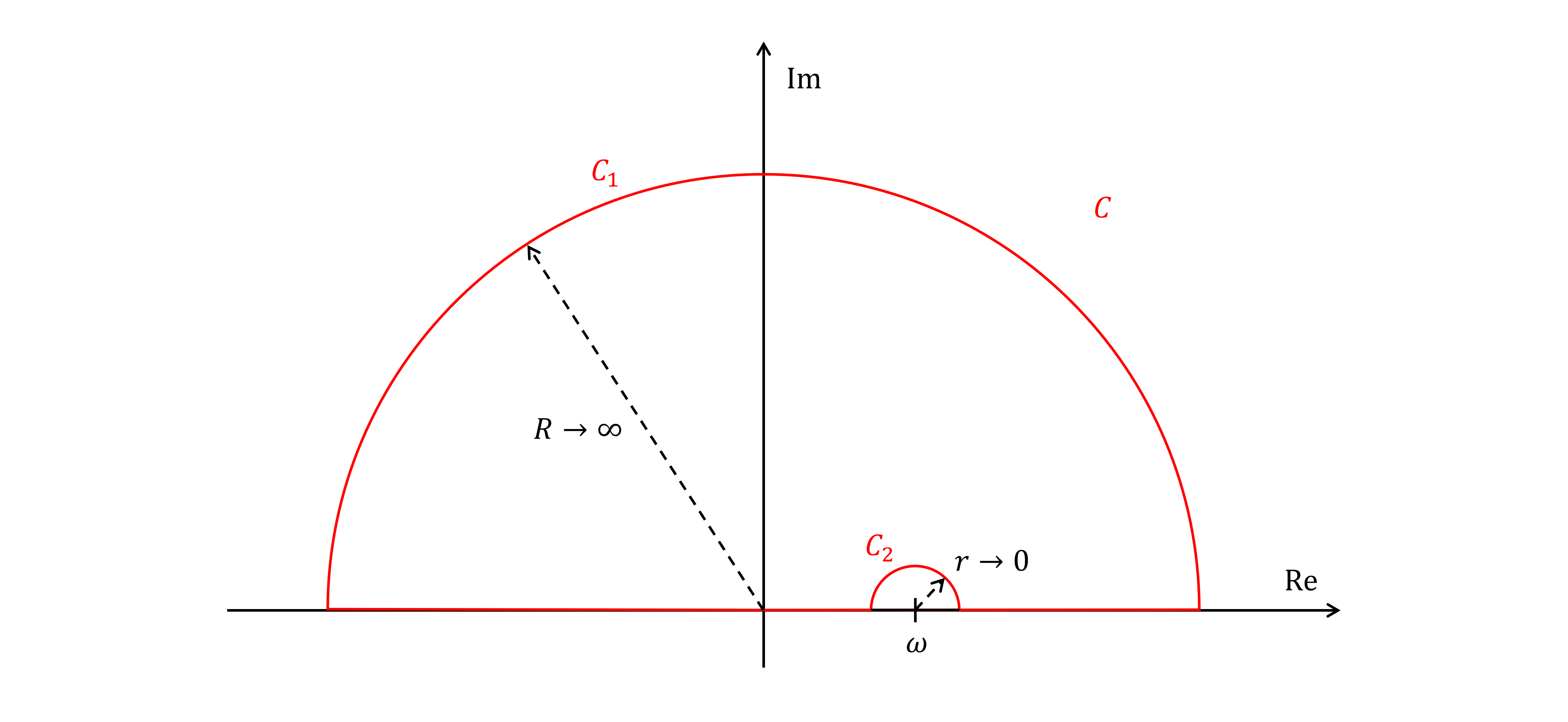
Figure 1 The contour $C$ to apply Cauchy's integral theorem on. $C$ consists of an infinitely large semicircle ($C_1$), an infinitesimally small semicircle around $z=\omega$ ($C_2$), and horizontal lines connecting the two semicircles on the real axis.

Applying Cauchy's integral theorem to the function $f(z) = \frac{\tilde\chi(z)}{z-\omega}$ and the contour $C$ as depicted in Figure 1, we obtain:

$$\oint_C {\frac{\tilde\chi(z)}{z-\omega}dz} = 0$$

The contour integral can be decomposed into each segment of the countour $C$ as follows:

$$\oint_C {\frac{\tilde\chi(z)}{z-\omega}dz} = \int_{C_1} {\frac{\tilde\chi(z)}{z-\omega}dz} + \int_{C_2} {\frac{\tilde\chi(z)}{z-\omega}dz} + \mathcal{P}\int_{-\infty}^{+\infty} {\frac{\tilde\chi(\omega')}{\omega'-\omega}d\omega'}$$

Here, the third term on the right-hand side is the principal value of the real-axis integral $\int_{-\infty}^{+\infty} {\frac{\tilde\chi(\omega')}{\omega'-\omega}d\omega'}$, defined as:

$$\mathcal{P}\int_{-\infty}^{+\infty} {\frac{\tilde\chi(\omega')}{\omega'-\omega}d\omega'} := \lim_{\epsilon \rarr 0+} \left[ \int_{-\infty}^{\omega-\epsilon} {\frac{\tilde\chi(\omega')}{\omega'-\omega}d\omega'} + \int_{\omega+\epsilon}^{+\infty} {\frac{\tilde\chi(\omega')}{\omega'-\omega}d\omega'} \right]$$

The first and second terms are each evaluated as:

$$\int_{C_1} {\frac{\tilde\chi(z)}{z-\omega}dz} = \lim_{R \rarr \infty} \int_{0}^{\pi} {\frac{\tilde\chi(Re^{i\theta})}{Re^{i\theta}-\omega}iRe^{i\theta}d\theta} = \int_{0}^{\pi}{i\lim_{R \rarr \infty} \tilde\chi(Re^{i\theta})}d\theta = 0$$

$$\int_{C_2} {\frac{\tilde\chi(z)}{z-\omega}dz} = \lim_{r \rarr 0+} \int_{\pi}^{0} {\frac{\tilde\chi(\omega+re^{i\theta})}{re^{i\theta}}ire^{i\theta}d\theta} = \int_{\pi}^{0}{i\tilde\chi(\omega)d\theta} = -i\pi \tilde\chi(\omega)$$

Plugging these results into the Cauchy's integral theorem, we obtain:

$$-i\pi \tilde\chi(\omega) + \mathcal{P}\int_{-\infty}^{+\infty} {\frac{\tilde\chi(\omega')}{\omega'-\omega}d\omega'} = 0$$

or

$$\tilde\chi(\omega) = \frac{1}{i \pi}\mathcal{P}\int_{-\infty}^{+\infty} {\frac{\tilde\chi(\omega')}{\omega'-\omega}d\omega'}$$

This equation yields the Kramers-Kronig relations between the real part and imaginary part of the electric susceptibility $\tilde\chi(\omega)$:

$$\mathrm{Re}\left[\tilde\chi(\omega)\right] = \frac{1}{\pi}\mathcal{P}\int_{-\infty}^{+\infty} {\frac{\mathrm{Im}\left[\tilde\chi(\omega')\right]}{\omega'-\omega}d\omega'}$$

$$\mathrm{Im}\left[\tilde\chi(\omega)\right] = -\frac{1}{\pi}\mathcal{P}\int_{-\infty}^{+\infty} {\frac{\mathrm{Re}\left[\tilde\chi(\omega')\right]}{\omega'-\omega}d\omega'}$$

Recalling that the relative permittivity $\varepsilon_r$ is related with electric susceptibility $\chi$ as $\varepsilon_r(\omega) = 1 + \tilde\chi(\omega)$, similar relations between the real and imaginary parts of the relative permittivity can be derived:

$$\mathrm{Re}\left[\varepsilon_r(\omega)\right] = 1 + \frac{1}{\pi}\mathcal{P}\int_{-\infty}^{+\infty} {\frac{\mathrm{Im}\left[\varepsilon_r(\omega')\right]}{\omega'-\omega}d\omega'}$$

$$\mathrm{Im}\left[\varepsilon_r(\omega)\right] = -\frac{1}{\pi}\mathcal{P}\int_{-\infty}^{+\infty} {\frac{\mathrm{Re}\left[\varepsilon_r(\omega') - 1 \right]}{\omega'-\omega}d\omega'}$$

Furthermore, the Kramers-Kronig relations can be derived for the complex refractive index $\tilde n(\omega) = n(\omega) - i\kappa(\omega)$, using the equation $\tilde n(\omega) = \sqrt{\varepsilon_r (\omega)} = \sqrt{1 + \tilde\chi (\omega)}$. Specifically, if we define a function $z \mapsto \tilde n(\omega) - 1 = \sqrt{1 + \tilde\chi(\omega)} - 1$, this function (i) is analytic and (ii) converges to zero as $z \rarr \infty$ in the LHP. Therefore, in the same way with the $\chi(\omega)$ case, we obtain the following relations between the real part - the refractive index $n(\omega)$, and the imaginary part - the extinction coefficient $\kappa(\omega)$, as follows:

$$n(\omega) = 1 + \frac{1}{\pi}\mathcal{P}\int_{-\infty}^{+\infty} {\frac{\kappa(\omega')}{\omega'-\omega}d\omega'}$$

$$\kappa(\omega) = -\frac{1}{\pi}\mathcal{P}\int_{-\infty}^{+\infty} {\frac{n(\omega') - 1}{\omega'-\omega}d\omega'}$$

Consequently, $n$ and $\kappa$ of a material are not independent: once the refractive index is given, the extinction coefficient is determined and vice versa. However, it is not practical to determine one of them from measurements on the other since the Kramers-Kronig relations require the measurement to be conducted on a wide range of frequency $\omega$. Thus, in practice, each of the quantities are usually measured independently.

The Lorentz Model for Permittivity and the Kramers-Kronig Relations

The Lorentz model, which models the electrons within a dielectric material as damped harmonic oscillators, states the frequency dependence of the relative permittivity as follows:

$$\varepsilon_r (\omega) = 1 + \frac{\omega_p^2}{(\omega_0^2-\omega^2) + i\gamma \omega}$$

The real and imaginary parts of the relative permittivity is derived from this equation as:

$$\mathrm{Re}\left[ \varepsilon_r(\omega) \right] = 1 + \frac{\omega_p^2 \left( \omega_0^2 - \omega^2 \right)}{\left( \omega_0^2 - \omega^2 \right)^2 + (\gamma\omega)^2}$$

$$\mathrm{Im}\left[ \varepsilon_r(\omega) \right] = \frac{\omega_p^2 \gamma \omega }{\left( \omega_0^2 - \omega^2 \right)^2 + (\gamma\omega)^2}$$

Since this solution of the Lorentz model is obtained from the physical system of a driven harmonic oscillator, it naturally satisfies the Kramers-Kronig relations.

This can also be checked by manually evaluating the integral. However, because the calculation is highly cumbersome, involving extensive partial fraction decomposition, it is left to the reader.